The final report can be downloaded here.

1. Implement a sum-product (SP) algorithm for decoding of the basic (15, 11) Hamming code.
   1. The function accepts LLRs from the channel, and provides the output L- values, representing the posterior distribution of the bits being 1 or 0.
   2. It may be an option to terminate the sum-product iterations early by verifying if all parity checks are satisfied.
   3. Compare the performance of the sum-product algorithm to that of the brute- force ML decoder of Exercise #2.
   4. What is the net coding gain (NGC) of the Hamming code under SP decoding?
2. Implement an LDPC decoder for the 5G LDPC base matrix B1 without puncturing at the basic rate of 1/3. The H matrix is provided separately, and for encoding, the Matlab toolbox may be used.
   1. Plot the BER vs SNR performance after the 1st, 2nd and 3rd iteration
   2. If simulation time allows, increase the number of iterations, until no further improvement in performance is possible. How many iterations are necessary to converge the performance?
   3. The capacity of the channel is given by Shannon in his famous formula \(C = 0.5 \cdot \log_2{(1 + SNR)}\), and is defined as the maximum ‘error-free’ achievable data rate by an ideal code. A capacity of 1/3 bits/symbol, which is the target of the turbo code, is achievable at an \(SNR= -2.3 \ dB \). What would you say about the turbo code?
   4. Assume ‘error-free’ to mean a BER lower than \(10^{−4}\). What are the gap to capacity and the net coding gain of the LDPC code at this BER?
3. Puncture the LDPC code to a rate of 2/3.
   1. Study the 5G standard and identify the puncturing scheme for the target rate.
   2. Perform decoding in a suitable SNR range in order to see a BER of \(10^{−4}\).
   3. What is the SNR required to reach a capacity of 2/3?
   4. What are the NCG and gap to capacity in this case?

Introduction

Low-Density Parity-Check Codes (LDPC) are a linear error correcting code, which is a method to transmit information over a noisy channel. LDPC (or Gallager code) is a block code that has a parity-check matrix, called H, which describes the linear relations of a codeword with its components. LDPC codes allow to the noise threshold to be set very close to the Shannon limit (the theorical limit) for a memoryless channel.

LDPC codes were invented in 1960 by Gallager at Massachusetts Institute of Technology. However, there was no practical decoding method at that time, LDPC codes were forgotten until 1996 which was rediscovered by David J. C. MacKay.

Given a channel output r, we wish to find the codeword t whose likelihood \(P(r \lvert t)\) is biggest. The best algorithm for low-density parity check codes known to perform an effective decoding is the sum-product algorithm. This algorithm is used to perform inference on graphical models. It calculates the marginal distribution for each unobserved node, conditional on any observer nodes.

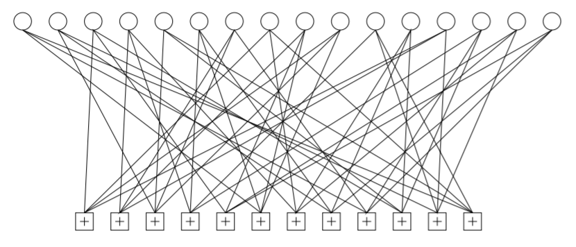
A regular LDPC code has a parity-check matrix, known as H, that has the same weigth j for every column and the same weight k for every row. This parity-check matrix can be seen graphically as in the next graph. In these example it is a code with \(j = 3\) and \(k = 4\), with \(N = 16\) variables and \(M = 12\) constraints. This parity check matrix defines the constrainst of the variables.

Theoretical part

Decoding with the sum-product algorithm in linear domain

To ilustrate this algorithm we will take a Hamming code (7,4). With a blocklength \(N = 7\), which the defines the code as a collection of N-tuples of symbols, and M the number of tuples (codewords) in this case \(M = 3\). The dimenstion of this code is \(K = 4\), which is the number of bits which are encoded. The code rate is defined as \(R = K / N = 4 / 7), that is the average entropy per symbol, it is related to its redundancy. Which means that K bits are encoded into N bits, adding M bits of redundancy. The parity-check matrix of our hamming code (7,4) is the following:

$$ H = \begin{bmatrix} 1 & 1 & 1 & 0 & 1 & 0 & 0 \\ 0 & 1 & 1 & 1 & 0 & 1 & 0 \\ 1 & 0 & 1 & 1 & 0 & 0 & 1 \end{bmatrix} $$

The parity-check matrix H has the same weight K for every row. It is possible to represent the parity-check matrix with the relations and the constraints of each bit as a factor graph. There are M check nodes or factors, that represent the constrains, are the blue squares. There are N variables represented as green circles that are the probability distributions of each transmitted bit. Each bit in our codeword participates in j constrains, that are the rows in our parity-check matrix. Each check node participates connects K bits. Each constraints forces the sum of the K bits to which it is connected to be even.

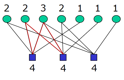
We can identify the set of bits that participate in check m by \(N(m) \equiv \{n : H_{mn} = 1\} \). The same way we define the set of checks in which bit n participates by \(M(n) \equiv \{m : H_{mn} = 1\} \). Some examples of these definitions:

$$ N(1) = \{1, 2, 3, 5\} \\ N(2) = \{2, 3, 4, 6\} \\ N(3) = \{1, 3, 4, 7\} \\ M(1) = \{1, 3\} \\ M(2) = \{1, 2\} \\ M(3) = \{1, 2, 3\} \\ M(4) = \{2, 3\} \\ M(5) = \{1\} \\ M(6) = \{2\} \\ M(7) = \{3\} \\ $$

There is also the shorthand \(M(n) \backslash m\) that denote the set with m element excluded, and \(N(m) \backslash n\) with the n element excluded.

The algorithm have two parts, q-messages denoted as \(q_{mn}\) and r-messages denoted as \(r_{mn}\). The value of \(q_{mn}^{x}\) is the probability that bit n of the word received has the value x, given the information obtained via check m. The value of \(r_{mn}^x\) is the probability of check m being satisfied if bit n of the word received is considered fixed to x and the other bits have a separable distribution given by the probabilities \(\{ q_{mn’} : n’ \in N(m) \backslash n \}\).

The algorithm consist in the next steps:

1. Initialize the q-messages
2. Horizontal step: Calculate r-messages with the q-messages
3. Vertical step: Calculate q-messages with the r-messages
4. Check the Halt condition with the pseudoposterior probabilities and the algorithm finishes if it satisfies the parity-check matrix, if not, repeat from step 2.

Initialization

In a Gaussian channel where the noise level varies in a known way the symbol likelihood is a Gaussian function. For every \((n,m)\) the variables \(q_{mn}^0\) and \(q_{mn}^1\) are initialized to the values of \(p_n^0\) and \(p_n^1\). As we are modelling our algorithm of a Gaussian channel, we initialize the q-messages as: $$ p_n^0 = q_{mn}^0 = \alpha_{mn} \cdot \exp{\big ( - \frac{1}{2 \sigma^2} \big( y_n - (-1) \big )^2 \big )} \\ p_n^1 = q_{mn}^1 = \alpha_{mn} \cdot \exp{\big ( - \frac{1}{2 \sigma^2} \big( y_n - (1) \big )^2 \big )} $$ Where \(y_n\) is the received signal, \(\sigma^2\) is the noise variance and \(\alpha_{mn}\) is a factor that makes \(q_{mn}^0 + q_{mn}^1 = 1\).

Horizontal step

In the horizontal step we run through the checks m and compute for each \(n \in N(m)\) two probabilities, \(r_{mn}^0\) and \(r_{mn}^1\). For \(r_{mn}^0\) it is the probability of the observe value when \(x_n = 0\), given that the other bits \(\{ x_{n’} : n’ \neq n \} \) have a separable distribution given by the probabilities \(\{ q_{mn’}^0 , q_{mn’}^1 \} \).
$$ r_{mn}^0 = \sum_{\{ x_{n’}: n’\in N(m) \backslash n \}} P(z_m \lvert x_n = 0, \{ x_{n’}: n’\in N(m) \backslash n \}) \prod_{n’\in N(m) \backslash n} q_{mn’}^{x_{n’}} \\ r_{mn}^1 = \sum_{\{ x_{n’}: n’\in N(m) \backslash n \}} P(z_m \lvert x_n = 1, \{ x_{n’}: n’\in N(m) \backslash n \}) \prod_{n’\in N(m) \backslash n} q_{mn’}^{x_{n’}} $$ The conditional probabilities in these summations are either zero or one, depending on whether the observed \(z_m\) matches the hypothesized values for \(x_n\) and the \(\{ x_{n’} \}\). The observed \(z_m\) matches when sum of the bits \(x_n\) and the \(\{ x_{n’} \}\) are even. As an example to ilustrate the previous expresion, for a factor that depends in variable \(f_1(x_2, x_3, x_5)\) we can define the \(r_{11}^0\) and \(r_{11}^1\) as:

$$ f_1(x_2, x_3, x_5) \rightarrow \\ r_{11}^{0} = p(b_2 = 0, b_3 = 0, b_5 = 0) + p(b_2 = 0, b_3 = 1, b_5 = 1) + \\ p(b_2 = 1, b_3 = 1, b_5 = 0) + p(b_2 = 1, b_3 = 0, b_5 = 1) \\ r_{11}^{1} = p(b_2 = 0, b_3 = 0, b_5 = 1) + p(b_2 = 0, b_3 = 1, b_5 = 0) + \\ p(b_2 = 1, b_3 = 0, b_5 = 0) + p(b_2 = 1, b_3 = 1, b_5 = 1) \\ $$

Vertical step

The vertical step takes the computed values of \(r_{mn}^0\) and \(r_{mn}^1\) and updates the values of the probabilities \(q^0_{mn}\) and \(q^1_{mn}\). For each n we compute:

$$ q^0_{mn} = \alpha_{mn} p_n^0 \prod_{m’\in M(n) \backslash m} r_{m’n}^0 \\ q^1_{mn} = \alpha_{mn} p_n^1 \prod_{m’\in M(n) \backslash m} r_{m’n}^1 $$ Where \(\alpha_{mn}\) is chosen such that \(q^0_{mn} + q^1_{mn} = 1\).

We can also compute the pseudoposterior probabilities \(q_n^0\) and \(q_n^1\)

$$ q^0_{n} = \alpha_{n} p_n^0 \prod_{m\in M(n)} r_{mn}^0 \\ q^1_{n} = \alpha_{n} p_n^1 \prod_{m\in M(n)} r_{mn}^1 $$

Halt condition

From the pseudoposterior probabilites the decoding procedure is the next.

$$ q_n^1 > 0.5 \Rightarrow v_n = 1 \\ q_n^1 \le 0.5 \Rightarrow v_n = 0 $$ Then we check if the decoded word satisfy the parity-check matrix. The multiplication with H give the syndrome as: $$ s = v H^{T} $$ If \(s = 0\) we can conclude that there are no errors, and we can finish with a successful decoding. If not, we have to go to the horizontal step until a maximum number of iterations is reached or the halt condition is satisfied.

Decoding with the sum-product algorithm in log domain

Linear domain, as presented in previous section, is difficult to implement due to all the variables you have to take into account. The previous algorithm can be solved with the ‘hyperbolic tangent’ increasing it performance and make it a simpler problem. As presented in linear domain, the low-density parity-check codes was expressed as \(q_{mn}^{0/1}\) and \(r_{mn}^{0/1}\). In log-domain it is replaced by the log probability-ratios \(l_{mn} \equiv \ln{q_{mn}^0 / q_{mn}^1} \). Thus, the algorithm is solved in a slightly different way.

The first step is Initialization. we initialize \(q_{mn}^{0}\) and \(q_{mn}^{1}\) using the log-likelihood ratio (LLR’s), we denote them as \(Lq_{mn}\).

$$ Lq_{mn} = - \frac{1}{2 \sigma^2} (y_n -1)^2 + \frac{1}{2 \sigma^2} (y_n + 1)^2 = \frac{2 y_n}{\sigma^2} \qquad y_n = \text{received signal} \\ $$ The horizontal step is solved with the hyperbolic tangent. We calculate \(Lr_{mn}\) as:

$$ Lr_{mn} = -2 \cdot atanh \prod_{n’ \in N(m) \backslash n} -\tanh{\frac{Lq_{m n’}}{2}} $$

The vertical step is solved as: $$ Lq_{mn}(x_n) = L_n + \sum_{m’ \in M(n) \backslash m} Lr_{m’ n} $$

In every iteration we can calculate the pseudoposterior probabilities as:

$$ Lq_n = Ln + \sum_{m’ \in M(n)} Lr_{m’ n} $$

From the pseudoposterior probabilities, \(Lq_n\), we can calculate a tentative decode as :

$$ Lq_n < 0 \rightarrow v_n = 0, \quad else: \quad v_n = 1 $$ As in linear domain, we check if the decoded word satisfy the parity-check matrix. The multiplication with H give the syndrome as: $$ s = v H^{T} $$ If \(s = 0\) we can conclude that there are no errors, and we can finish with a successful decoding. If not, we have to go to the horizontal step until a maximum number of iterations is reached or the halt condition is satisfied.

5G standard

5G is the fifth generation technology standard for broadband cellular networks. It is the successor of the 4G replacing convolutional and turbo codes with polar and low-density parity-check (LDPC) codes. The properties of LDPC such as incremental redundancy, hardware friendly, high net coding gain, makes them perfect for 5G communications. This protocol is designed to have rate compatibility and a variable code length.

In the 5G specification [22, 5.3.2], there are two types of base graphs whose usage is determined by code rate or a size of information bits. The base-graph is constructed using quasi-ciclic method, replacing each zero-value entry with a \( Z \ \times \ Z \) all-zero matrix and each non-zero valued entry with \( Z \ \times \ Z \) permutation matrix. The base graph can be considered as codes whose permutation is only allowed to be circular shift. This greatly reduces the memory requirement for implementation while also facilitating the use of a simple switch network for encoding and decoding. The 5G defines 15 different liftinng sizes, \(Z_c\), and there are eight different permutation matrix designs per base graph.

The input bit sequence to the code block segmentation is denoted by \(b_0, b_1, b_2, b_3, \ … \ , b_{B−1} \), where \(B>0\). If \(B\) is larger than the maximum code block size \(K_{cb}\), segmentation of the input bit sequence is performed and an additional CRC sequence of \(L=24\) bits is attached to each code block. For LDPC base graph 1, the maximum code block size is \(K_{cb}=8448\). For LDPC base graph 2, the maximum code block size is \(K_{cb}=3840\). The lifting size must be \(K = 22 Z_c\) for base graph 1 and \(K = 10 Z_c\) for base graph 2. The bits output from code block segmentation are denoted by \(c_{0}, c_{1}, c_{2}, c_{3}, \ … \ , c_{K−1} \), where \(K\) is the number of bits for the code block. After encoding the bits are denoted by \(d_0, d_1, d_2, \ …. \ , d_{N-1}\) where \(N = 66 Z_c\) for LDPC base graph 1.

5G LDPC codes support rate matching functionality to select and arbitrary amount of transmitted bits.The minimum code rate of the encoding and decoding graph is limited at 2/3 while base graph 1 itself can support the code rate as low as 1/3.

Implementation

An implementation of the LDPC codes was made using MatLab. Two implementations are proposed, one in linear domain and other in log domain. The implementation in linear domain has big perfomance faults, and we will use it as a way to understand the sum-product algorithm. The log domain algorithm is optimized to work with big codes, as the implementation in 5G.

Some common functions are defined that will be used in the both implementations. This functions are regarded to the operations\(N(m) \equiv \{n : H_{mn} = 1\} \), \(M(n) \equiv \{m : H_{mn} = 1\} \), \(M(n) \backslash m\) and \(N(m) \backslash n\).

function M_n = M_n(n, H)
    M_n = find(H(:, n) == 1)';
end

function M_n_m = M_n_m(n, m, H)
    M_n_m = find(H(:, n) == 1);
    M_n_m = M_n_m(M_n_m ~= m)';
end

function N_m = N_m(m, H)
    N_m = find(H(m, :) == 1);
end

function N_m_n = N_m_n(m, n, H)
    N_m_n = find(H(m, :) == 1);
    N_m_n = N_m_n(N_m_n ~= n);
end

In order to test the algorithm, a random data word is generated and encoded with a hamming code. The data is going to transmited in a Additive Gaussian white noise channel. This is simulated in matlab using the function randn. The hamming code is generated using the matlab built-in function hammgen. The encoded data is modulated using BPSK, that is transmitting -1 and 1. In the next code it is showed how the data is transmitted into the channel.

m = 4
N = 2^m-1
K = N - m

% generate parity check matrix and generator matrix using Matlab functions
[H,G] = hammgen(m);

% Random transport block data generation
data = randi(\[0 1\], 1, K)

% Hamming encoding
encoded = mod(data*G, 2) % using generator matrix

% Noise
SNR = 10^(1/10);
noiseVar = 1/SNR;

% BPSK
modulated = 2*(encoded)-1

% AWGN
noise = sqrt(noiseVar/2)*randn(size(modulated))
chOut = modulated + noise % channel output

Implementation in linear domain

The following implementation is a direct interpretation of the sum-product algorithm in linear domain of the theory presented above. This solution has problems in performance, but it is a good example to ilustrate how the sum-up algorithm works. The steps followed are the same as showed previously: initialization, horizontal step, vertical step and halt condition.

The algorithm starts with the initialization of the q-messages. The \(q_{mn}^{0/1}\) are initializated as a Gaussian function.

q_0 = zeros(m, N); % Initialize matrix
q_1 = zeros(m, N);
alpha = zeros(m, N);

for n_i = 1:length(chOut)
    q_0(:, n_i) = exp(-(1/(2*noiseVar)) * (chOut(n_i) - (-1))^2);
    q_1(:, n_i) = exp(-(1/(2*noiseVar)) * (chOut(n_i) - (1))^2);
    
    alpha(:, n_i) = 1 / (q_0(1, n_i) + q_1(1, n_i));
    
    q_0(:, n_i) = q_0(:, n_i) * alpha(1, n_i);
    q_1(:, n_i) = q_1(:, n_i) * alpha(1, n_i);
end

% Calculate prior probability
p_0 = q_0(1,:)
p_1 = q_1(1,:)

In the horizontal step we iterate in the \(m\) and \(n\) values and we calculate the r-messages. From the equation showed in the horizontal step, the conditional probabilities are either zero or one, depending if the observed \(z_m\) matches the checks, which is when the sum of the bits \(x_n\) and \(\{x_{n’} \}\) are even. This operation is synthesize in matlab as:

r_0 = zeros(m, N);
r_1 = zeros(m, N);

for m_i = 1:m
    for n_i = 1:N
        n_pri = N_m_n(m_i, n_i, H); % set
        
        % All the possible combinations of
        % bits from the previous set
        % Go to every combination of the past set
        for comb_i = 0:(2^size(n_pri, 2))-1
            % Check operation, sum the numbers of 1's
            % The observed z_m matches when sum of the bits x_n and the x_{n'} are even
            if ~mod(sum(de2bi(comb_i) == 1 ), 2)
                r_0(m_i, n_i) = r_0(m_i, n_i) + prod_prob(n_pri, comb_i, q_0, q_1, m_i);
            else
                r_1(m_i, n_i) = r_1(m_i, n_i) + prod_prob(n_pri, comb_i, q_0, q_1, m_i);
            end
        end
    end
end

In the last piece of code it is used the function prod_prob, which is a function that calculate the product of the probabilities given the position of the bits. This function was used to make it easier the calculation of r-messages.

function prod_prob = prod_prob(bit_pos_set, bit_values, prob_0, prob_1, m)
    % Compute the products of probabilities given a set of bit positions,
    % the value of those bits in decimal format, the matrix for being 0 of
    % those bits and the matrix for being 1 of those bits
    
    prod_prob = 1;

    for i = 1:length(bit_pos_set)
        bi_bit_values = de2bi(bit_values, length(bit_pos_set)); % to binary
        if bi_bit_values(i)
            %disp("Testing p = 1 of " + bit_pos_set(i))
            prod_prob = prod_prob * prob_1(m, bit_pos_set(i));
        else
            %disp("Testing p = 0 of " + bit_pos_set(i))
            prod_prob = prod_prob * prob_0(m, bit_pos_set(i));
        end
    end 
end

Then in the vertical step we calculate the q-messages from the r-messages and the prior probabilities. It is performed as:

for n_i = 1:N
    for m_i = 1:m
        q_0(m_i, n_i) = p_0(n_i);
        q_1(m_i, n_i) = p_1(n_i);
        
        m_pri = M_n_m(n_i, m_i, H);
        
        for i = 1:length(m_pri)
            q_0(m_i, n_i) = q_0(m_i, n_i) * r_0(m_pri(i), n_i);
            q_1(m_i, n_i) = q_1(m_i, n_i) * r_1(m_pri(i), n_i);
        end
        
        alpha(m_i, n_i) = 1 / (q_0(m_i, n_i) + q_1(m_i, n_i));
        
        q_0(m_i, n_i) = q_0(m_i, n_i) * alpha(m_i, n_i);
        q_1(m_i, n_i) = q_1(m_i, n_i) * alpha(m_i, n_i);
    end
end

At this point it is posible to get the pseudo posterior distributions to get a tentative deconding:

% Initialize pseudoposterior probabilities
pse_q_0 = zeros(1, N);
pse_q_1 = zeros(1, N);
pse_alpha = zeros(1, N);

for n_i = 1:N
    pse_q_0(n_i) = p_0(n_i);
    pse_q_1(n_i) = p_1(n_i);
    m_pri = M_n(n_i, H);
    
    for i = 1:length(m_pri)
        pse_q_0(n_i) = pse_q_0(n_i) * r_0(m_pri(i), n_i);
        pse_q_1(n_i) = pse_q_1(n_i) * r_1(m_pri(i), n_i);
    end
    
    pse_alpha(n\_i) = 1 / (pse_q_0(n_i) + pse_q_1(n_i));
    pse_q_0(n_i) = pse_q_0(n_i) * pse_alpha(n_i);
    pse_q_1(n_i) = pse_q_1(n_i) * pse_alpha(n_i);
end

At this point of the code we can go back to the horizontal step and iterate the algorithm until the halt condition is satisfied. With the pseudo posterior probabilities we can have a tentative decoding and multiply it with the parity-check matrix to get the number of errors. If the number of errors is 0 we can finish the algorithm, if not we continue to the horizontal step. The halt condition is calculated as:

% Check exit condition
v = pse_q_0 <= 0.5;

errors = sum(mod(v * H', 2)); %Numbers of erros
disp("Number of errors " \+ errors)

Implementation in log-domain

The previous section it is presented the implementation for linear domain. Although it is a direct translation of the equations presented in the theoretical part, its performance for big codes is really bad. Modern transceivers works in log-domain based in the increase of performance. In this section it is presented an implementation of the sum-product algorithm in log-domain. This algorithm is optimized for big codes and tested for 5G. The steps followed are the same than presented earlier: initialization, horizontal step, vertical step and halt condition.

First we start with the initialization of the q-messages using the log-likelihood ratio (LLR) from the received message:

% Calculate the log-likelihood ratio (LLR's)
LLR = 2/noiseVar*chOut

% Initialize lq messages with LLR in every row
lq = repmat(LLR,m, 1);

% Calculate prior probability, that is the input LLR's
l_n = LLR

The horizontal step is calculated as moving horizontally (every column in the parity-check matrix) and calculting the set of \(N(m)\). In the 5G parity-check matrix, with size of 17664x26112, a check is only connected with 30 variables as much, this means that the calculation of the operation \(N(m) \backslash n\) is in most of the cases is \(N(m)\). To improve the performance of the algorithm in big codes, we are not iterating with variables and the checks, m and N, otherwise, we are iterating the over the constraints and over the variables that this constraints are connected. This way, the algorithm is faster as we don’t have a double loop iterating the checks and the variables, in this case, only iterate through the checks.

lr = zeros(m, N);

for m_i = 1:m
    n_i_set = find(H(m_i, :) ~= 0); %N_m
    
    % Calculate the product outside the loop
    % to save calculations
    prod_n_i_set = prod(-tanh(lq(m_i, n_i_set) / 2));
    lr_n_i_set = -2 * atanh(prod_n_i_set);
    lr(m_i, :) = lr_n_i_set;
    
    for n_i = 1:length(n_i_set)
        n_pri = n_i_set(n_i_set ~= n_i_set(n_i)); % N_m_n
        prod_n_pri = prod(-tanh(lq(m_i, n_pri) / 2));
        lr(m_i, n_i_set(n_i)) = -2 * atanh(prod_n_pri);
    end
end

In the vertical step a similar approach, as in the horizontal step, is followed. In this case we iterate over the rows of the parity-check matrix, iterating the variables, and we only visit the constraints in which these variables are connected. The code is the next one.

for n_i = 1:N
    m_i_set = find(H(:,n_i) ~= 0);
    lq(:, n_i) = sum(lr(m_i_set,n_i)) + l_n(n_i);
    
    for m_i = 1:length(m_i_set)
        m_pri = m_i_set(m_i_set ~= m_i_set(m_i));
        lq(m_i_set(m_i), n_i) = sum(lr(m_pri,n_i)) + l_n(n_i);
    end
end

We can get the pseudo posterior probabilities to get a tentative decoding similar to the linear domain.

% Calculate pseudoposterior probabilities
for n_i = 1:N
    m_pri = M_n(n_i, H);
    
    pse_lq(n_i) = l_n(n_i) + sum(lr(m_pri, n_i));
end

The last step is to check the halt condition. As in linear domain, the algorithm keep iterating, going back to the horizontal step, until the halt condition is reached. In the next piece of code we perform a tentative decoding and we calculate the number of errors. In case the number of errors is 0 we finish the decoding process, otherwise we continue with the horizontal step.

% Check exit condition
v = pse_lq >= 0; % 0 if < 0

% Calculate numbers of errors
errors = sum(mod(v * H', 2)); %Numbers of erros

Simulation results

First exercise

1. Implement a sum-product (SP) algorithm for decoding of the basic (15, 11) Hamming code.
   1. The function accepts LLRs from the channel, and provides the output L- values, representing the posterior distribution of the bits being 1 or 0.
   2. It may be an option to terminate the sum-product iterations early by verifying if all parity checks are satisfied.
   3. Compare the performance of the sum-product algorithm to that of the brute- force ML decoder of Exercise #2.
   4. What is the net coding gain (NGC) of the Hamming code under SP decoding?

The code used for this exercise is presented in the previous section, using the log-domain to solve the problem. The code used is uploaded here. It is peformed the creation of 10000 different random binary packets, and then transmitted in a additive white Gaussian noise channel. Different algorithm are tested in order to compare the capabilities of the sum-product algorithm. The output graph:

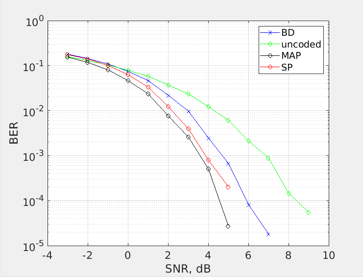
The sum-product algorithm is better thatn the bound-distance algorithm, giving a gain of 0.5 dB for a BER of \(10^{-3}\). The SP algorithm is better for big messages, in this scenario where the messages are encoded with 15 bits, the performance of the sum-product algorith does not stand out too much. The net coding gain of the sum-product algorithm is about 3 dB for a BER of \(10^{-3}\). Its performance is very close to the theorical limit.

Second exercise

2. Implement an LDPC decoder for the 5G LDPC base matrix B1 without puncturing at the basic rate of 1/3. The H matrix is provided separately, and for encoding, the Matlab toolbox may be used.
   1. Plot the BER vs SNR performance after the 1st, 2nd and 3rd iteration
   2. If simulation time allows, increase the number of iterations, until no further improvement in performance is possible. How many iterations are necessary to converge the performance?
   3. The capacity of the channel is given by Shannon in his famous formula \(C = 0.5 \cdot \log_2{(1 + SNR)}\), and is defined as the maximum ‘error-free’ achievable data rate by an ideal code. A capacity of 1/3 bits/symbol, which is the target of the turbo code, is achievable at an \(SNR= -2.3 \ dB \). What would you say about the turbo code?
   4. Assume ‘error-free’ to mean a BER lower than \(10^{−4}\). What are the gap to capacity and the net coding gain of the LDPC code at this BER?

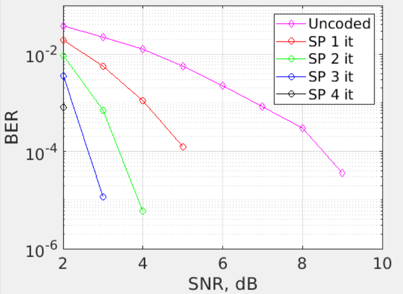
The code used for this section is uploaded here. The implementation is slighly different from the previous version, but adapted to use for different iterations of the sum-product algorithm. With the matlab toolbox of 5G it is easy to work with 5G. In the course materials it is given the functions to generate the parity-check matrix or base-graph known in the 5G standard. The function used to generate the base graph is retrieve_H_5G_NR_simple. Then we generate different packages of 8448 random bits, and encode them using the matlab function nr5g.internal.ldpc.encode. As defined in the 5G standard normally the encoder ouput corresponding to the first two columns of the base graph is not transmitted, this is translated into the code by assign the LLR values of those positions to 0. However, in this exercise we are not performing any puncturing to the data. We are going to perform a BER vs SNR plot for the 1st, 2nd, 3rd and 4th iteration:

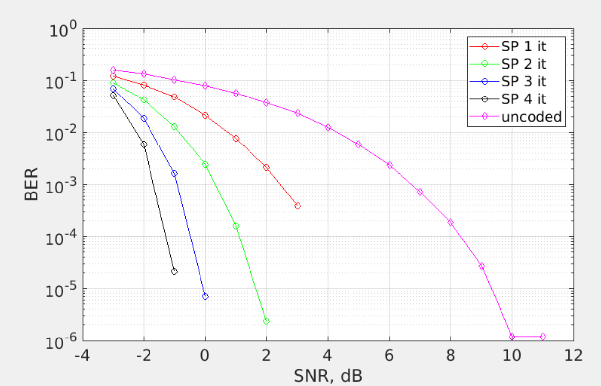
From the plot from above there is no further improvement in performance after 4 iterations, there is an improvement, but the computational cost and the results after the 4 iterations make it not worthwhile to perform further iterations. The performance of LDPC codes are very good for high noise channels, giving a results near to the theorical limit given by shannon. The capacity of a channel is given by Shannon in his famous formula \(C = 0.5 \cdot \log_2{(1 + SNR)}\), for a capacity of 1/3 bits/symbol is achievable at an \(SNR= -2.3 \ dB \). At an SNR of \(-2.3 \ dB \) it is obtained a BER of \(10^{-2}\) with 4 iterations, which is a really good result.

The gap to capacity obtained for LDPC codes with 5G in this exercise is \(1 \ dB\) for 4 iterations, \(1.8 \ dB \) for 3 iterations and \( 3.4 \ dB \) for 2 iterations. Moreover, the net coding gain is \(9.6 \ dB \) for 4 iterations, \(8.8 \ dB \) for 3 iterations, \(7.2 \ dB \) for 2 iterations and \( 4.7 \ dB \) for one iteration. These results states the capabilities of LDPC codes, and its use in 5G communications is quite successful.

Third exercise

3. Puncture the LDPC code to a rate of 2/3.
   1. Study the 5G standard and identify the puncturing scheme for the target rate.
   2. Perform decoding in a suitable SNR range in order to see a BER of \(10^{−4}\).
   3. What is the SNR required to reach a capacity of 2/3?
   4. What are the NCG and gap to capacity in this case?

5G LDPC codes support rate matching functionality to select and arbitrary amount of transmitted bits.The minimum code rate of the encoding and decoding graph is limited at 2/3 while base graph 1 itself can support the code rate as low as 1/3. The base graph used in the previous section, the parity-check matrix for 5G communicacions, can be used for rate 2/3 without any modifications. To perform this change in the rate we need to puncture, that means not transmitting, the last \(3/2 \cdot 8448 \) bits of the data after the encoder. Then, in the receiving process, we need to fix the LLR of those bits to 0, becuase the information we have about those bits in reception is \(LLR = \log{(p (y \lvert x = 1))} / \log{(p (y \lvert x = 0))} = 0\). We are going to repeat the same exercise as in the previous section but with another rate, and also puncturing the correspoding bits. The code used for this section is uploaded here. It is generated a BER vs SNR plot for different iterations of the sum-product algorithm. The results are not very accurate because it was performed using 20 blocks for each SNR levec, causing that the resolution of the graph is not the best. This happen because of lack of time for simulation.

The SNR required to reach a capacity of 2/3 is:

$$ C = 0.5 \cdot \log_{2}{(1+ SNR)} \\ C = 2 / 3 \Rightarrow SNR = 1.81 \ dB $$ Assuming that ‘error-free’ is obtained with a BER of \(10^{-4}\), the gap to capacity obtained in this exercise are \(0.7 \ dB\) for 3 iterations, \(1.7 \ dB\) for 2 iterations and \(3.2 \ dB\) for 1 interation. The net code gain of LDPC for 2/3 rate is \(5.8 \ dB\) for 3 iterations, \(4.8 \ dB\) for 2 iterations and \(3.3 \ dB\) for 1 iteration. Comparing these results, using a rate of 2/3 by puncturing the data, with the results in the previous section, using rate 1/3 without puncturing, we can see that the net code gain is negatively affected with the puncturing. In the case of gap to capacity in these two cases, the results are better after the puncturing, but these results doesn’t make sense and the reason is that this simulation was run with less block codes than in the previouse section, without puncturing. This generate that the resolution is this section is not as good as in the graph without puncturing. The expected results of the gap to capacity in the both sections must be that it should be higher without puncturing than with puncturing, at least 0.5 dB in 3 iterations.

Conclusions

LDPC codes shows to be a really good algorithm in channel with high noise. From the exercise above we can see its performance with low SNR. The capabilities of this codes are impresive. Rate matching