$$ E = \text{Electric Field} = [Volts / m] \\ H = \text{Magnetic Field} = [A / m] \\ D = \text{Electric flux density} = [C / m^2] \\ B = \text{Magnetic flux density} = [T] \\ M = J_m = \text{Magnetic current density} = [Volts / m^2] \\ J_e = \text{Electric current density} = [A / m^2] \\ A = \text{Magnetic vector potential} = [Volts \cdot s / m] \\ F = \text{Electric vector potential} = [A \cdot s / m]\\ $$

$$ D = \epsilon E \\ B = \mu H $$

Where:

• \(\epsilon\): Electric permittivity
• \(\mu\): Magnetic permeabilitty

Basic operations

$$ \text{Gradient} \qquad \nabla V = \frac{\partial V}{\partial x} \hat u_x + \frac{\partial V}{\partial y} \hat u_y + \frac{\partial V}{\partial z} \hat u_z \\ \text{Divergence} \qquad \nabla \cdot \vec A = \frac{\partial A_x}{\partial x} + \frac{\partial A_y}{\partial y} + \frac{\partial A_z}{\partial z} \\ \text{Curl} \qquad \nabla \times \vec A = \Big ( \frac{\partial A_z}{\partial y} - \frac{\partial A_y}{\partial z} \Big ) \hat u_x + … \\ \text{Laplace operator or Laplacian} \qquad \nabla^2 V = \frac{\partial^2 V}{\partial x^2} + \frac{\partial^2 V}{\partial y^2} + \frac{\partial^2 V}{\partial z^2} $$

In spanish Curl is “Rotacional”.

Other relations of vector operators:

$$ \nabla \times (\nabla V) = 0 \\ \nabla \cdot (\nabla \times A) = 0 $$

Maxwell Equations - Simple Materials

$$ \nabla \times E = - \mu \frac{\partial H}{\partial t} - J_m \qquad \text{Faraday’s law} \\ \nabla \times H = \epsilon \frac{\partial E}{\partial t} + J_e \qquad \text{Ampère-Maxwell’s law} \\ \nabla \cdot E = \frac{\rho_e}{\epsilon} \qquad \text{Gauss’law (electric)} \\ \nabla \cdot H = \frac{\rho_m}{\mu} \qquad \text{Gauss’law (magnetic)} \\ \nabla \cdot B = 0 $$

Where:

$$ \epsilon = \text{Permittivity} \\ \mu = \text{Permeability} $$

In a isotropic linear homogeneous medium it is defined:

$$ D = \epsilon E + P \\ H = \frac{B}{\mu} $$

Maxwell equations . Time-Harmonic case

To avoid heavy notations it is used phasor domains.

A real field is expressed in the following way:

$$ E(r, t) = E_0(r) \cos{[\omega t +\alpha(r) ]} $$ We can use phasor to get rid of the phase of the signal:

$$ E(r, t) = Re[E_0(r)e^{j\alpha(r)}e^{jwt}] = Re[E(r)e^{j\omega t}] $$ This way:

$$ \frac{\partial}{\partial t} \rightarrow j\omega $$

And the maxwell equations can be expressed as:

$$ \nabla \times E = - j \omega \mu H - J_m \qquad \text{Faraday’s law} \\ \nabla \times H = j \omega \epsilon E + J_e \qquad \text{Ampère-Maxwell’s law} \\ \nabla \cdot E = \frac{\rho_e}{\epsilon} \qquad \text{Gauss’law (electric)} \\ \nabla \cdot H = \frac{\rho_m}{\mu} \qquad \text{Gauss’law (magnetic)} $$

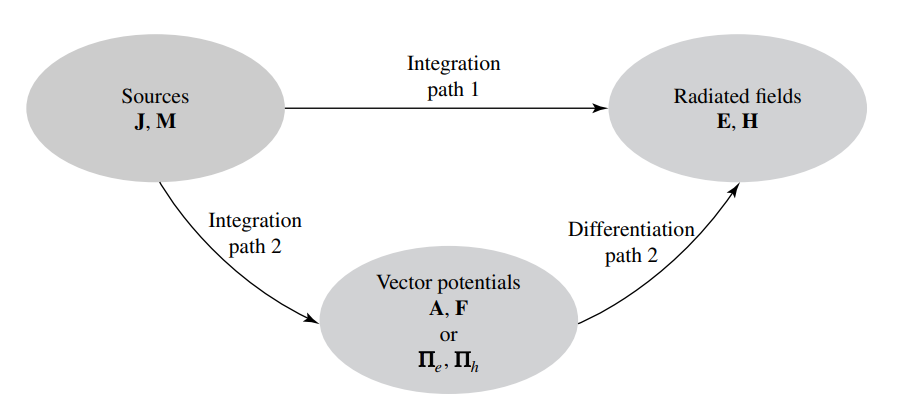
Radiation integrals and auxiliary potential functions

$$ J = J_e = \text{Electric Current density} = [Amperes / m^2] \\ M = J_m = \text{Magnetic current density} = [Volts / m^2] \\ E = \text{Electric Field} = [Volts / m] \\ H = \text{Magnetic Field} = [A / m] \\ A = \text{Magnetic vector potential} = [Volts \cdot s / m] \\ F = \text{Electric vector potential} = [A \cdot s / m]\\ $$

Boundary conditions

$$ a_{n2} \times (E_1 - E_2) = - J_{m,s} \\ a_{n2} \times (H_1 - H_2) = J_{e,s} \\ a_{n2} \cdot (D_1 - D_2) = \rho_{e,s} \\ a_{n2} \cdot (B_1 - B_2) = \rho_{m,s} \\ $$ The tangencial component of the electric field is discontinious if \(J_{m, s} \neq 0\) The tangencial component of the magnetic field is discontinious if \(J_{e, s} \neq 0\) The normal component of the electric flux density is discontinious if \(\rho_{e, s} \neq 0\) The normal component of the electric flux density is discontinious if \(\rho_{m, s} \neq 0\)

Where \(a_{n2}\) is the unitary vector perpendicular to the surface that goes from medium 1 to medium 2.

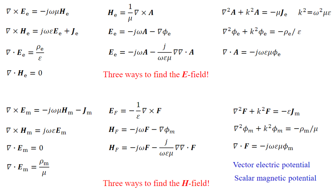
Vector and scalar Potentials I

From the maxwell equations we can define them for a electrical source and a magnetic source:

$$ X = X_e + X_m $$

In the electrical source the equations are defined as:

$$ \nabla \times E_e = - j \omega B_e \qquad \text{Faraday’s law} \\ \nabla \times H_e = j \omega D_e + J_e \qquad \text{Ampère-Maxwell’s law} \\ \nabla \cdot D_e = \rho_e \qquad \text{Gauss’law (electric)} \\ \nabla \cdot B_e = 0 \qquad \text{Gauss’law (magnetic)} $$ In a magnetic source the equations are defined as:

$$ \nabla \times E_m = - j \omega B_m - J_m \qquad \text{Faraday’s law} \\ \nabla \times H_m = j \omega D_m \qquad \text{Ampère-Maxwell’s law} \\ \nabla \cdot D_m = 0 \qquad \text{Gauss’law (electric)} \\ \nabla \cdot B_F = \rho_m \qquad \text{Gauss’law (magnetic)} $$

Vector and scalar potentials

$$ \nabla \cdot B_e = 0 \Leftrightarrow B_e = \nabla \times A $$ The expression above comes from: $$ \nabla \cdot B_e = 0 = \nabla \cdot (\nabla \times A) \Rightarrow B_e = \nabla \times A $$ Substituting in the Maxwell equation we get that:

$$ E_A = - \nabla \phi_e - j \omega A $$ Where the scalar function \(\phi_e\) represents an arbitrary electric scalar potential which is a function of position

Lorenz’ condition:

$$ \nabla \cdot A = - j \omega \epsilon \mu \phi_e $$

$$ A = \frac{\mu}{4 \pi} \int \int_V \int J \frac{e^{-jkR}}{R} dv' $$

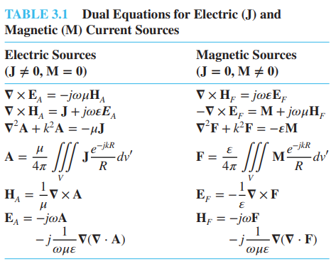
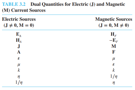
Duality theorem

When two equations that describe the behavior of two different variables are of the same mathematical form, their solutions will also be identical. The variables in the two equations that occupy identical positions are known as dual quantities and a solution of one can be formed by a systematic interchange of symbols to the other. This concept is known as the duality theorem.