The key of the first part is that all bodies emit radiation because of the temperature. Known as the back boddy radiation.
Planck’s law: Radiation, or spectral radiance of a body, is defined as. In this course is defined as brighness. It can be expressed as B or P:
$$ B_{bb} = \frac{2 h f^3}{c^2} \frac{1}{e^{hf/kT_p}-1} $$
$$
[B] = \frac{W}{m^2 \cdot Sr \cdot Hz}
$$

The radio band of microwave is really linear in B.
In microwave region we use the 1st order taylor approximation -> Rayleigh-Jeins=>
$$ B_{bb} \approx \frac{2hf^3}{c^2}\frac{k T_p}{hf} = \frac{2 k T_p}{\lambda^2} \\ k \rightarrow \text{Boltzman} $$

$$ B = B_{bb} \cdot e \\ e = \text{emmisivity} , e \in [0,1] $$
In a Radiometer we are measuring that radiation. A black body absorbs all the radioation, and it can radiate all its energy, it is the most absorbent and the opposite. A white buddy reflects all the radiation, like silver (not perfect). Blackbody has e = 1, polished silver plate has e = 0
Boundary conditions
Grey bodies are physical bodies. If we look to a grey body, it cannot generate more energy than received:
$$ B_{gb} = e_x \ B_{bb} \\ e_x = \text{emissivity (transmittivity)} \\ x = \text{polarization} \\ e_x \in [0,1] $$ As an example of a plane surface. We can calculate the radiation with the Fresnel Formula: $$ e_v = 1 - r_v \\ r_v = \text{Radiation} = \Big \lvert \frac{\Epsilon_r \cos{\theta} - \sqrt{\Epsilon_r - \sin^2{\theta}}}{\Epsilon_r \cos{\theta} + \sqrt{\Epsilon_r - \sin^2{\theta}}} \Big \lvert^2 $$ Where \(\Epsilon\) is the permitivity. With that we can know what type of material is in front, without toaching it. It is a stochastic proccess => Comes with a standard deviation.
It is defined the brightness temperature, or apparant temperature of the object, that is:
$$ B_{bb} = \frac{2k}{\lambda^2} T_p \\ B_{gb} = B_{bb} \cdot e_x = \frac{2k}{\lambda^2} \cdot e_x \cdot T_p \\ T_B = \text{Object brightness temperature} = e_x \cdot T_p $$ ¿How to get from brightness to power?
 T_B is a stochastic signal. It expresses power, given by the Rayleigh-Jeans approximation to Planc’s Radiation Law, P = k•B•T, where k = 1.23•10-23 J/K is Boltzmanns constant, B is the bandwidth, and T is the temperature.
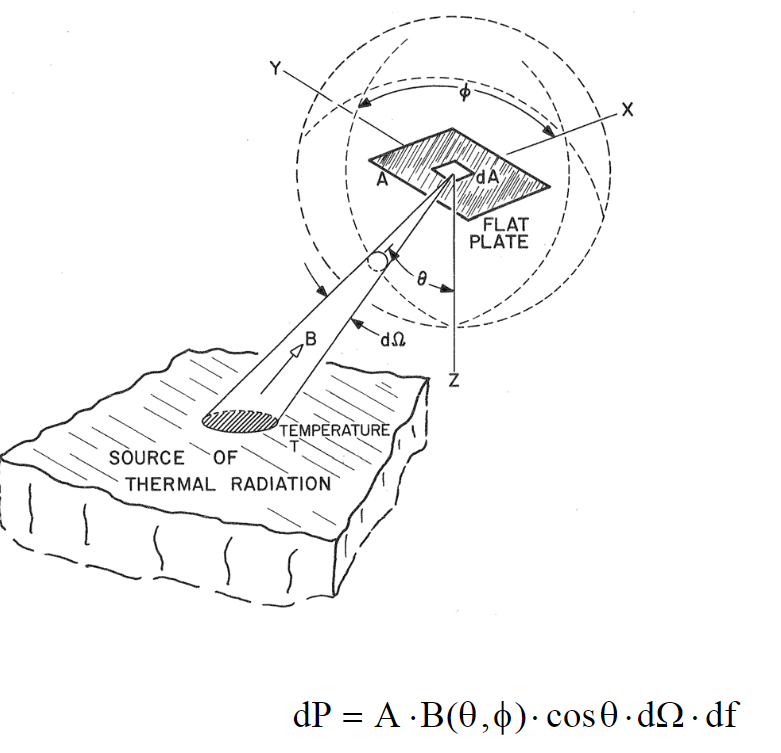
$$ dP = A \cdot B(\theta, \phi) \cdot \cos{\theta} \cdot d \Omega \cdot d f $$
B is brightness, A is area, f is frequency. That is the power contribution of thermal radiation of an object. This equation can be complicated when integrating the angle. The power is received by an antenna, that is way different from a plate. Where \(d\Omega\) is the angle, a point.
Antennas introduction - Radiometry approach
Some theory about antennas that I am going to skip. The normalized field pattern is a dimensionless number with maximum value of unity
The received power at the antenna will be:
$$ dP = B(\theta, \phi) \cdot A_e{\theta, \phi} \cdot d\Omega \cdot d f $$
\(A_e\) is the effective area of the antenna. Integrate to get P. As we dont know the input signal we are going to use circular polarization. Using horizontal/vertical polarization is an error because if it is perpendicular we dont receive power, with circular polarization we loss the 50%, that is why the 1/2 in the equation:
$$ P = \frac{1}{2} \int_{f_{min}}^{f_{max}} \Big ( \int \int_{4 \pi} B(\theta, \phi) \cdot A_e(\theta, \phi) \cdot d\Omega \Big ) df $$ The brightness is an abstract quantity but it gives us information of the material we are receiving. We can express this a bit different:
$$ P = \frac{1}{2} \frac{2k}{\lambda^2} \frac{\lambda^2}{4 \pi} \int_{f_{min}}^{f_{max}} \Big ( \int \int_{4 \pi} T_B(\theta, \phi) \cdot G(\theta, \phi) \cdot d\Omega \Big ) df \\ BW = f_max - f_min \Rightarrow P = K \cdot BW \cdot \Big ( \frac{1}{4 \pi} \int \int_{4 \pi} T_B(\theta, \phi) \cdot G(\theta, \phi) \cdot d\Omega \Big) \\ = K \cdot BW \cdot T_A \\ T_A = \text{Gain weighted average of } T_B’s \text{ around the antenna} \\ T_A = \frac{1}{4 \pi} \int \int_{4\pi}G(\theta, \phi) \cdot T_B(\theta, \phi) d\Omega $$ The received signal is passive, and stochastic. Stochastic means that we need to extend our measurement over time in order to get the signal, also means that the signal comes with a standard deviation. The standard deviation is:
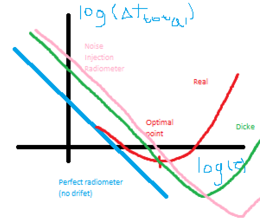
$$ \Delta T = \frac{T_A + T_N}{\sqrt{B \cdot \tau}} \qquad \text{Radiometric resolution} $$
Building a radiometer
This type of radiometer are defined as Total Power Radiometer (TPR)
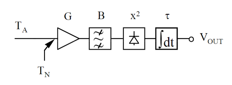 Ideally at the output we have:
$$ V_o = k \cdot B \cdot G \cdot T_A $$ However the amplifier will generate noise temperature \(\T_N): $$ V_o = k \cdot B \cdot G (T_A + T_N) $$ As the noises are random and independant, the average is going to be 0. G and T_N vary over time and need calibration, 2 calibration points are needed.
Radiometer calibration
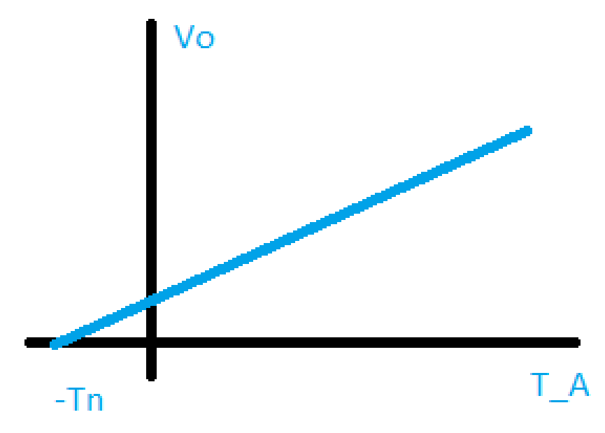
You put the antenna in objects that you know that output. The radiometer calibration consist in finding the line. Some objects that can be used for the calibration process:
- Use a black body
- Microwave absorber at different temperatures
- Matched microwave termination at different temperatures
- Point the antenna into space. But the problem on these is the atmosphere attenuation.
- Use a “noise diode” = constant current diode. The problem is that it adds Ti (T inyected) on top of Ta.
Things that you need to be aware of:
- Radiometric resolution
- Component drifts (G and Tn) Calbiration accuracy drops over time
- Transmission line losses
The transmission line losses, where \(\gamma\) are the losses in dB:
$$ T’_A = T_A(1 - \gamma) + \gamma \cdot T_p \\ T_p = \text{Physical temperature} $$
Radiometer configurations
- TPR Defined above
Dicke Radiometer (DR)
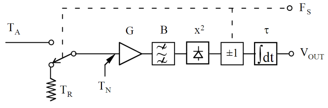
Switch between the antenna and something we know (a match load), we can substract from each other, and we have a relative measurement. F_s is the switching frequency, ej 1 KHz.
In half of the perior the Vout will be:
$$ V_o = K \ B \ G \ (T_R + T_N) $$ In the other half of the period:
$$ V_o = K \ B \ G \ (T_A + T_N) $$ In total after the subraction we have:
$$ V_o = K \ B \ G \ (T_R - T_A) $$
Where:
- \(T_N\) is eliminated
- G errors are reduced.
- Only 1 calibration point neede
However the radiometric resolution is lower:
$$ \Delta T = 2 \cdot \frac{T_A + T_N}{\sqrt{B \cdot \tau}} $$
Noise injection Radiometer (NIR)
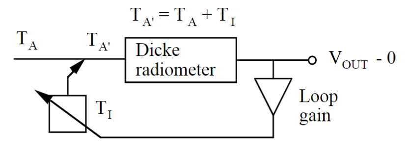
$$ V_{out} = c \cdot (T’_A - T_R) \cdot G \approx 0 $$
$$ T_I = D \cdot T’_I \qquad D = \text{Duty cycle} \\ T_A = T_R - T_I = T_R - T’_D \cdot D $$
$$ \Delta T = 2 \cdot \frac{T_A + T_N}{\sqrt{B \cdot \tau}} $$
Where:
- No calibration points are needed
- G is also eliminated
Hybrid Radiometer
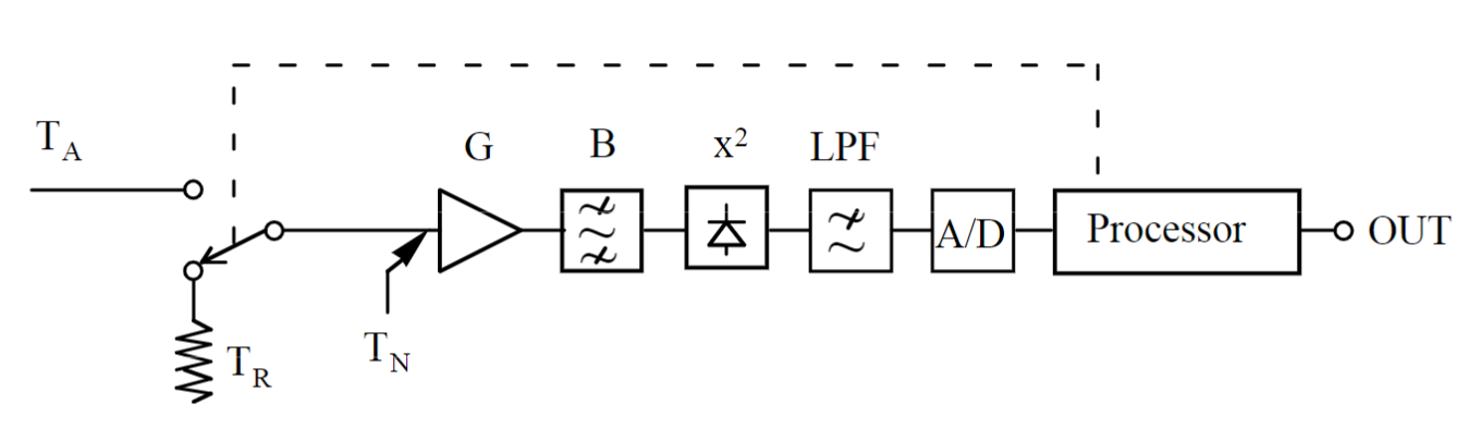
Similar at the others, but this time using a FPGA or something similar.