Constellation diagram

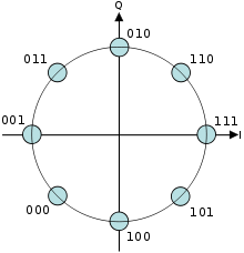
A constellation diagram is used to represent symbols for QAM and PSK. It is composed by the horizontal axis (“I” in phase), in which the and vertial axis (“Q” in quadrature, shifted 90º). The amplitude is the distance between the symbol and the origin, and the phase is the angle with the horizontal axis.

QAM modulation

QAM modulation:

$$ s_k (t) = I_k \cdot p(t) \cdot \cos{(\omega_0 t)} - Q_k \cdot p(t) \cdot \sin{(\omega_0 t)} $$

In which:

• p(t) is a 1 or 0, the data
• \(I_i\) and \(Q_i\) can be discrete values (possible values) equispaced and symmetrically distributed around 0.

Basically QAM is the sum between a sinus and a cosine, the cos the horizontal axis and sinus the vertical axis in the constellation diagram.

Also it can be written as:

$$ x = A (\cos{(2 \pi f t + \phi_0)} + j \sin{(2 \pi f t + \phi_0)}) = A e^{j(2 \pi f t + \phi_0)} = A_1 \cos{(2 \pi f t + \phi_0)} + j A_2 \sin{(2 \pi f t + \phi_0)} \\ A = \sqrt{A_1^2 + A_2^2} \\ \phi_0 = arc tan - \frac{A_1}{A_2} $$

So, the modulation can be represented as:

$$ x = A_1 + j A_2 $$

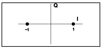
BPSK

BPSK is equivalent to:

$$ x = A_1 + j A_2 \\ A_1 = \pm 1 \\ A_2 = 0 \\ \Rightarrow 1 \Rightarrow \phi_0 = + \pi, A_1 = 1 \\ \Rightarrow 0 \Rightarrow \phi_0 = - \pi, A_1 = 1 $$

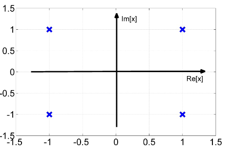
4QAM or QPSK

$$ x = A_1 + j A_2 \\ A_1 = \pm 1 \\ A_2 = \pm 1 \\ \Rightarrow 00 \Rightarrow 1 + i\\ \Rightarrow 01 \Rightarrow -1 + i \\ \Rightarrow 10 \Rightarrow -1 -i \\ \Rightarrow 11 \Rightarrow +1 - i $$

Hard decisions and soft decisions

• Hard decisions are finding the word with less errors, that is, to compare the received data with the H (parity check matrix) and find the word with less errors.
• Soft decisions is to find the word with the most correlation with our codeword.

In matlab hard decision would be:

% Random transport block data generation        
        data = randi([0 1], 1, K);
        % Hamming encoding
        encoded = mod(data*G, 2); % using generator matrix

        % BPSK
        modulated = 2*(encoded)-1;

        % AWGN
        noise = sqrt(noiseVar/2)*randn(size(modulated));
        chOut = modulated + noise; % channel output
        % LLR. Needed in following exercises
        LLR = 2/noiseVar*chOut;
        
        % hard decision using bounded distance
        withErrors = chOut > 0;
        % BD decoding using Matlab's function
        decData = decode(withErrors, N, K, 'hamming/binary');
        newBER_BD = sum(decData ~= data) / K; % count the errors on the information bits
        BER_BD(ii) = BER_BD(ii) + newBER_BD; % BER

Which is generating a random word, encoding it with hamming code, modulate in BPSK (+1 for 1 and -1 for 0), adding noise, and then taking the hard decision to bit per bit put if it is higher than 0, and then get the numbers of errors in the decoder.

With the soft decision would be:

% ML soft decision
        % compare the channel output to all possible codewords, and chose
        [~, decodedIdx] = min(sum(abs(repmat(chOut, 2^K, 1) - allCodewords).^2, 2));
        % the one with the minimum ED as optimal
        decBitsMAP = allDataCombos(decodedIdx, :);
        newBER_MAP = sum(decBitsMAP ~= data) / K;
        BER_MAP_SD(ii) = BER_MAP_SD(ii) + newBER_MAP;

Which consist in generate a matrix with a copy of the channel output, then substract each column with the codeword… and then get the minimum of the sum of each row. This is a way to get the word that is the most likely to our codewords. In other words is to substrat the channel output with our codewords and get the one that get less error.

1. Simulate an AWGN channel in the range of SNR = [0; 8] dB (specified per symbol!) with a BPSK modulation.
   1. The input should be encoded using the Hamming code (15, 11)
   2. Calculate the BER of the encoded bits before performing decoding and plot it against the SNR
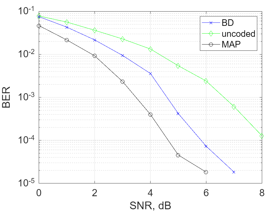
2. Perform decoding using the bounded distance decoder from Exercise 1. Plot the results together with the uncoded BER from question 1. How much is the coding gain at the target BER of 10−3? What about the net coding gain (which is obtained by subtracting the extra power needed to transmit the parity bits)?
3. Implement a MAP decoder for the Hamming code. The MAP is implemented by calculating the Euclidean distance of the received real-valued vector to all codewords of the code (of which there are 211, so implementation speed matters here. If the program is too slow, revert to the (7, 11) code instead).
4. How much gain is there from soft-decision MAP w.r.t. the bounded distance decoder at the target BER of 10−3?

clc
close all
clear all

m = 4;
N = 2^m-1;
K = N - m;
% generate parity check matrix and generator matrix using Matlab functions
[H, G] = hammgen(m);
% generate all possible codewords for comparison later
if m <= 4
    allDataCombos = de2bi(0:2^K-1);
    allCodewords = 2*mod(allDataCombos*G, 2)-1;
end
    
nBlocks = 10000;

SNRAll = [0:1:8]; % in dB
BERuncoded = zeros(1, length(SNRAll));
BER_MAP_SD = zeros(1, length(SNRAll));
BER_BD = zeros(1, length(SNRAll));

for ii = 1:length(SNRAll)
    fprintf('simulating.. SNR = %.1f dB \n', SNRAll(ii));
    
    SNR = 10^(SNRAll(ii)/10);
    noiseVar = 1/SNR;
    for nn = 1:nBlocks
        % Random transport block data generation        
        data = randi([0 1], 1, K);
        % Hamming encoding
%         encoded = encode(data, N, K,'hamming/binary'); % using Matlab
        encoded = mod(data*G, 2); % using generator matrix

        % BPSK
        modulated = 2*(encoded)-1;

        % AWGN
        noise = sqrt(noiseVar/2)*randn(size(modulated));
        chOut = modulated + noise; % channel output
        % LLR. Needed in following exercises
        LLR = 2/noiseVar*chOut;
        
        % hard decision using bounded distance
        withErrors = chOut > 0;
        % BD decoding using Matlab's function
        decData = decode(withErrors, N, K, 'hamming/binary');
        newBER_BD = sum(decData ~= data) / K; % count the errors on the information bits
        BER_BD(ii) = BER_BD(ii) + newBER_BD; % BER
        
        % ML soft decision
        % compare the channel output to all possible codewords, and chose
        [~, decodedIdx] = min(sum(abs(repmat(chOut, 2^K, 1) - allCodewords).^2, 2));
        % the one with the minimum ED as optimal
        decBitsMAP = allDataCombos(decodedIdx, :);
        newBER_MAP = sum(decBitsMAP ~= data) / K;
        BER_MAP_SD(ii) = BER_MAP_SD(ii) + newBER_MAP;
        
        % uncoded BER
        BERuncoded(ii) = BERuncoded(ii) + sum((LLR(N-K+1:N) > 0) ~= data) / K;
    end
end

BER_BD = BER_BD / nBlocks;
BERuncoded = BERuncoded / nBlocks;
BER_MAP_SD = BER_MAP_SD / nBlocks;

semilogy(SNRAll, BER_BD, '-bx', SNRAll, BERuncoded, '-gd', SNRAll, BER_MAP_SD, '-ko')
grid on
legend('BD', 'uncoded', 'MAP');
xlabel('SNR, dB');
ylabel('BER')
set(gca, 'fontsize', 16);

And the output is the following: