GNSS time series analysis for referenceframes
When we establish a referenceframe we need to determine how that referenceframe is connected to a parent referenceframe. One of the key tasks is to determine the velocity of the referencesystem (i.e. the benchmarks and the GNSS stations) with respect to the parent referenceframe.
We will therefore explore the time evolution of two GNSS stations. The first GNSS station, situated in Denmark, exhibit primarily liniar motion in the up direction due to post glacial uplift. The second GNSS station, situated in Japan close to the Fukushima Nuclear power plant, exhibit a post seismic displacement.
A key asumption for the reference system is that the velocity of benchmarks and station is constant over time.
Start by importing some usefull Python tools for time series analysis.
import pandas as pd
import numpy as np
import matplotlib.pyplot as plt
import math
1 The buddinge station
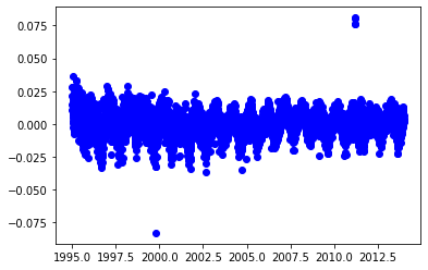
Use Pandas to import positon residuals from the Buddinge station in Copenhagen. To get an overview of the timeseries we plot the $\delta up$ component (dU) as a function of time and construct a line showing the theoretical average of the residual uppening.
budpRes = pd.read_csv('dBUDP_10101M003_ULR6B.neu',
                      sep='\s+', comment='#', header=None,
                      names=['year', 'dN', 'dE', 'dU', 'SDN', 'SDE', 'SDU'])

plt.scatter(budpRes['year'], budpRes['dU'], color='blue')

yearSpan = np.array([budpRes['year'].iloc[0], budpRes['year'].iloc[-1]])
upSpan = np.array([0.0, 0.0])

plt.plot(yearSpan, upSpan, color='red')
plt.show()

1.1 Determine the up velocity
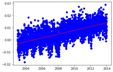
For the Buddinge station we only expect to see a simple liniar uplift over time. Assume that the up motion can be described using a simple linear equation:
$$y=a+bx$$
or in matrix form
$$ Y = A\cdot b\\ \left[\begin{array}{c} y_0 \\ y_1 \\ y_2 \\ \vdots \\ y_n \end{array}\right]= \left[\begin{array}{cc} 1 & x_0 \\ 1 & x_1 \\ 1 & x_2 \\ \vdots & \vdots \\ 1 & x_n \\ \end{array}\right] \left[\begin{array}{c} a\\ b \end{array}\right] $$
We can now find the best estimate of $a$ and $b$ using least squares:
$$b=(A^TA)^{-1}A^T Y$$
First we extract the data columns we are going to use and setup the A matrix. Next we estimate the unknow b vector using the Moore-Penrose Matrix.
y = budpRes['dU'].to_numpy()
x = budpRes['year'].to_numpy()
A = np.concatenate((np.ones((x.shape[0], 1)),
                    x.reshape((x.shape[0],1))),
                    axis=1)         # Construct the A matrix from a column of 1's and a column with x values

At = A.T                            # Example: the transposed of A
MP = np.linalg.inv(At.dot(A))       # Example: the inverse of (At * A)

b = np.zeros(2)            # placeholder for print and plot
b = MP.dot(At).dot(y)      # Implement the above function

print(f"Uplift rate {b[1]} m/y")

upFit = A.dot(b)

plt.scatter(x, y, color='blue')
plt.plot(x, upFit, color='red')
plt.show()
Uplift rate 0.001548826525655773 m/y
1.2 Determine the up velocity in the presens of a discontinuity
We are now looking at the second GNSS station, situated in Japan close to the Fukushima Daiini Nuclear power plant. During the earthquake the staion “jumps” to a new position followed by a long period with post seismic displacement while the crust adjust to the new situation.
The earthquake happend on March 11 2011, and we therfore start by plotting the GNSS timeseries for a period before and after the earthquake.
tskbRes = pd.read_csv('dTSKB_21730S005_ULR6B.neu',
                      sep='\s+', comment='#', header=None,
                      names=['year', 'dN', 'dE', 'dU', 'SDN', 'SDE', 'SDU'])
plt.scatter(tskbRes['year'], tskbRes['dU'], color='blue')

yearSpan = np.array([tskbRes['year'].iloc[0], tskbRes['year'].iloc[-1]])

timeEQ = 2011.0 + 70.0 / 365.0

timeSpanEQ = np.array([timeEQ, timeEQ])
upSpan = np.array([-0.09, 0.03])

plt.plot(timeSpanEQ, upSpan, color='black')       # Plot earthquake time
plt.show()
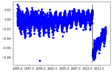
We can see that in addition to the simple linear up motion prior to the earthquake there is also a post seismic deformation after the earthquake, that we can asume to be linear. Remember that we asume that the velocity of the benchmarks and stations in the reference system is constant over time.
$$y_{psd}=a_{psd}+b_{psd}x$$
We can therefore split the motion into two parts.
1: Before the earthquake:
$$y=a+bx$$
2: and after the earthquake:
$$y=a + a_{psd} + bx + b_{psd}x$$
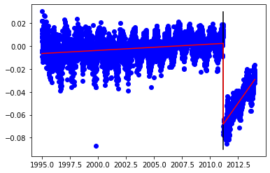
Let $_e$ be the time of the earthquake (or last observation just before) and combining the two on matrix form:
$$ Y = A\cdot b\ \left[\begin{array}{c} y_0 \\ y_1 \\ y_2 \\ \vdots \\ y_e \\ y_{e+1} \\ \vdots \\ y_n \end{array}\right]= \left[\begin{array}{cccc} 1 & 0 & x_0 & 0 \\ 1 & 0 & x_1 & 0\\ 1 & 0 & x_2 & 0\\ \vdots & \vdots & \vdots & \vdots \\ 1 & 0 & x_e & 0 \\ 0 & 1 & x_{e+1} & x_{e+1} \\ \vdots & \vdots & \vdots & \vdots \\ 0 & 1 & x_n & x_n \end{array}\right] \left[\begin{array}{c} a\\ a_{psd}\\ b\\ b_{psd} \end{array}\right] $$
Solution is found as before:
$$b=(A^TA)^{-1}A^T Y$$
tskbUpBefore = tskbRes.loc[tskbRes['year'] <= timeEQ, 'dU']
tskbUpAfter = tskbRes.loc[tskbRes['year'] > timeEQ, 'dU']

y = tskbRes['dU'].to_numpy().reshape(tskbRes.shape[0], 1)
x = tskbRes['year'].to_numpy().reshape(tskbRes.shape[0], 1)

A = np.zeros((len(x), 4))                       # placeholder for print and plot

A = np.concatenate((np.ones((x.shape[0], 1)),
                    x.reshape((x.shape[0],1))),
                    axis=1)         # Construct the A matrix from a column of 1's and a column with x values

# Get moment of earthquake e
samples_sep = x[2] - x[1]
e = math.floor((timeEQ - x[0]) / (samples_sep))

first_col = np.concatenate((np.ones((e, 1)), np.zeros((x.shape[0]-e, 1))), axis = 0)
sec_col = np.concatenate((np.zeros((e, 1)), np.ones((x.shape[0]-e, 1))), axis = 0)
fourth_col = np.concatenate((np.zeros((e, 1)), x[e:]), axis = 0)

A = np.concatenate((first_col, sec_col, x.reshape((x.shape[0],1)), fourth_col), axis=1)

At = A.T                            # Example: the transposed of A
MP = np.linalg.inv(At.dot(A))       # Example: the inverse of (At * A)

b = np.zeros(2)            # placeholder for print and plot

b = MP.dot(At).dot(y)      # Implement the above function

print('Station up bias before: {:.3f} m'.format(b[0][0]))  # you need [0][0] to get before bias i.e first row
print('Station up bias after: {:.3f} m'.format(b[1][0]))
print('Station up velocity: {:.3f} mm/year'.format(1000.0 * b[2][0]))
print('Station PSD velocity: {:.3f} mm/year'.format(1000.0 * b[3][0]))
Station up bias before: -1.092 m
Station up bias after: -27.942 m
Station up velocity: 0.544 mm/year
Station PSD velocity: 13.316 mm/year
plt.scatter(x, y, color='blue')
plt.plot(timeSpanEQ, upSpan, color='black')

upFit = A.dot(b)
plt.plot(x, upFit, color='red')
plt.show()
Residuals
We can now remove the modelled station velocity and psd motion and evaluate the residuals.
res = y - upFit
plt.scatter(x, res, color='blue')
plt.show()