- Muchas notas - Fran Acién

Assignment 3A

%% Section 1.1
% Author Francisco Jesús Acién Pérez-
% Place on the Retrack directory

fnL1 = dir('CS_OFFL_SIR_SAR_1B_20131206T230535_20131206T230712_B001.DBL');
fnL2 = dir('CS_OFFL_SIR_SAR_2A_20131206T230535_20131206T230712_B001.DBL');
[HDR1, CS2]=Cryo_L2_read(fnL2.name);
[HDR, CS] =Cryo_L1b_read(fnL1.name);

lightvel = 2.9979E8;

%% Section 1.2

% There are 110 signals

wwf_1Hz=squeeze(CS.AVG.data);

waveform_num=40;

waveform = wwf_1Hz(:,waveform_num)';
x=1:1:length(waveform);


figure(1)
plot(x, waveform);     % Plot 40

%% Section 1.3

A=max(waveform);  % Max_amplitude

Pn = (1/5)*sum(waveform(1:5));

Th=Pn + 0.8*(A - Pn);


%% Section 1.4

delGate=0;

for i = 1:length(wwf_1Hz(waveform_num,:))
    if waveform(i) >= Th
        delGate = i;
        break
    end
end

sprintf("Retrackted decimal gate is %d", delGate)
deltaGateSeconds = delGate* 3.12;

Ttracker = CS.AVG.win_delay(waveform_num)*1E9;
T = deltaGateSeconds + Ttracker;    % In ns
range = (lightvel * (T*1E-9))/2;

%% Section 1.4.2

ranges = zeros(1,length(wwf_1Hz(1,:)));
for signal = 1:length(wwf_1Hz(waveform_num,:))
    waveform = wwf_1Hz(:,signal)';
    A=max(waveform);  % Max_amplitude

    Pn = (1/5)*sum(waveform(1:5));

    Th=Pn + 0.8*(A - Pn);
    delGate=0;

    for i = 1:length(waveform)
        if waveform(i) >= Th
            delGate = i;
            break
        end
    end
    
    deltaGate = delGate*3.12;

    Ttracker = CS.AVG.win_delay(signal)*1E9;
    T = deltaGate + Ttracker;    % In ns
    ranges(signal) = (lightvel * (T*1E-9))/2;
end

%% Section 1.5

corr((CS.COR.corr_status.dry_trop>0),1) = CS2.COR.dry_tropo;
corr((CS.COR.corr_status.wet_trop>0),1) = corr+CS2.COR.wet_tropo;
corr((CS.COR.corr_status.gim_iono>0),1) = corr+CS2.COR.iono;
corr((CS.COR.corr_status.dac>0),1) = corr+CS2.COR.inv_baro;
corr((CS.COR.corr_status.ocean_equilibrium_tide>0),1) = corr+CS2.COR.ocean_tide;
corr((CS.COR.corr_status.solidearth_tide>0),1) = corr+CS2.COR.solid_earth;
corr((CS.COR.corr_status.geocentric_polar_tide>0),1) = corr+CS2.COR.geoc_polar;

rangesC = ranges + corr';

%% Q2

waveform_num = 1;

for i = 1:length(corr)
    if abs(corr(i)) >= abs(corr(waveform_num))
        waveform_num = i;
    end
end

sprintf("Largest value of correction is %d", waveform_num)

%% 1.6 - Q3

H_RangeC = zeros(1, length(rangesC));       % SSH
for range = 1:length(rangesC)
    H = CS.AVG.H(range);
    H_RangeC(range) = H - ranges(range);
end

%% 1.7 - Q4

SLA_1Hz = H_RangeC - CS2.COR.mss_geoid';

beginning_index = 10;
last_index = length(SLA_1Hz);

figure(2)
plot(CS.AVG.lat(beginning_index:last_index), SLA_1Hz(beginning_index:last_index));

Q1. Plot waveform 40 and report how your retracked decimal gate (for waveform 40).

Waveform 40 has the next form:

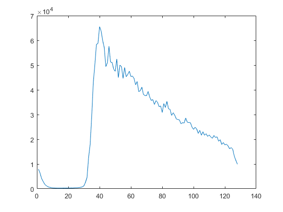
The Retrackted decimal gate is 38, that is when the power exceed the threshold of 80% of max power.

Q2. Which correction has the largest magnitude.

waveform_num = 1;

for i = 1:length(corr)
    if abs(corr(i)) >= abs(corr(waveform_num))
        waveform_num = i;
    end
end

sprintf("Largest value of correction is in waveform %d", waveform_num)

Largest value of correction is in waveform 84.

Q3. Compute SSH for all waveforms using: H-RangeC

H_RangeC = zeros(1, length(rangesC));       % SSH
for range = 1:length(rangesC)
    H = CS.AVG.H(range);
    H_RangeC(range) = H - ranges(range);
end

Q4. A. Create a plot of SLA_1Hz as a function of Latitude.

SLA_1Hz = H_RangeC - CS2.COR.mss_geoid';

beginning_index = 10;
last_index = length(SLA_1Hz);

figure(2)
plot(CS.AVG.lat(beginning_index:last_index), SLA_1Hz(beginning_index:last_index));

The plot is the next one:

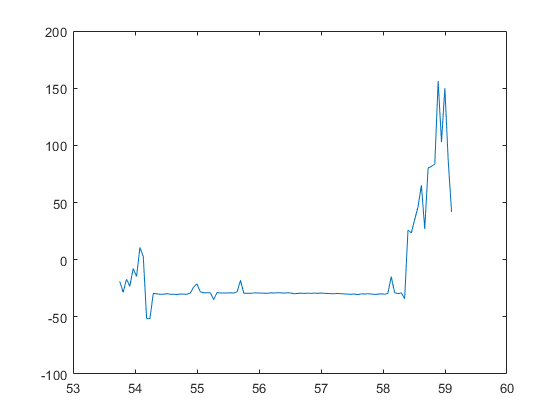
There is a surge roughly from waveform 40 to 86. The magnitude of this surge is 1.36771 m.

Assignment 3B

MSS, Geoid and MDT in the North Sea and in the Baltic Sea.

Use the altimetry.dat which is part of the retrack.zip archive above. File contains 1 Hz Satellite observations in 7 columns: Format(1: track,2:latitude,3:long,4: MDT, 5: Dummy, 6: Geoid, 7: MSS)

Q1:Create Plot of the MSS and MDT for the (54-67N and 0E-35E) region using i.e. plot3 or scatter function.

Its nice if you can get plot_google_map to work, but I have not tested if it work and its not mandatory (script is attached in retracking.zip).

# Load telemetry

class Altimetry:
    def __init__(self, track, latitude, long, MDT, Dummy, Geoid, MSS):
        self.track = float(track)
        self.latitude = float(latitude)
        self.long = float(long)
        self.MDT = float(MDT)
        self.Dummy = float(Dummy)
        self.Geoid = float(Geoid)
        self.MSS = float(MSS)

f = open("altimetry.dat")

lines = f.readlines()

observations = []

lines[0].split()

for line in lines:
    data = line.split()
    observations.append(Altimetry(data[0], data[1], data[2], data[3], data[4], data[5], data[6]))

import matplotlib.pyplot as plt
from mpl_toolkits.mplot3d import axes3d

fig1 = plt.figure()
fig2 = plt.figure()
ax_mss = fig1.add_subplot(111, projection='3d')
ax_mdt = fig2.add_subplot(projection='3d')

xs = []
ys = []
zs_mss = []
zs_mdt = []

for observation in observations:
    #print("LAT: {:.2f} LONG: {:.2f}".format(observation.latitude, observation.long))
    if(observation.latitude >= 54 and observation.latitude <= 67 and
       observation.long >= 0 and observation.long <=35):
        xs.append(observation.latitude)
        ys.append(observation.long)
        zs_mss.append(observation.MSS)
        zs_mdt.append(observation.MDT)
ax_mss.scatter(xs, ys, zs_mss, s=0.1)
#ax_mss.view_init(270, 0)

ax_mdt.scatter(xs, ys, zs_mdt, s=0.1)
#ax_mdt.view_init(270, 0)
plt.show()

png

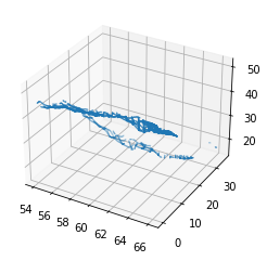
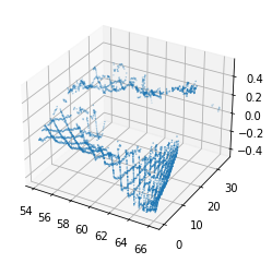
Q2: Which satellite do you think is used (Jason, ERS/ENVISAT or both)

We can see that it is a JASON satellite due to the inclination of the pass

Determine the MSS, Geoid and MDT for the following three locations and determine the difference in MSS, Geoid and MDT between the following three locations (you can not find these directly. Just use any nearby location):

Point 1: 57.5N, 5E (Central North Sea).
Point 2: 55.0 7.0E (Close to Denmark)
Point 3: 57.5N, 20E (Baltic Sea).

Q3: Report the 3 values in the 3 locations in a table.

def print_nearby_points(lat, long, offset):
    p1_latitude = lat
    p1_long = long

    square_offset = offset

    study = []

    for observation in observations:
        if(observation.latitude >= p1_latitude - square_offset and observation.latitude <= p1_latitude + square_offset and
           observation.long >= p1_long - square_offset and observation.long <= p1_long + square_offset):
            study.append(observation)

    for data in study:
        print("LAT: {:.3f} LON: {:.3f} MSS: {:.3f} MDT: {:.3f} Geoid: {:.3f}".format(data.latitude, data.long, data.MSS, data.MDT, data.Geoid))
        
print("POINT 1")
print_nearby_points(57.5, 5, 0.14)

print("\nPOINT 2")
print_nearby_points(55, 7, 0.2)

print("\nPOINT 3")
print_nearby_points(57.5, 20, 0.08)

POINT 1
LAT: 57.363 LON: 5.077 MSS: 42.534 MDT: 0.049 Geoid: 42.484

POINT 2
LAT: 55.194 LON: 6.833 MSS: 41.242 MDT: 0.124 Geoid: 41.119

POINT 3
LAT: 57.548 LON: 20.050 MSS: 22.064 MDT: 0.363 Geoid: 21.701

Q4:

What do you think the Geoid to be higher in point 1 than 3?

The influence of Spredningszoner in the atlatic sea.

What do you think the MDT to be higher in point 2 than 1 ?

Because of the North Atlantic Drift.

What do you think causes the MDT to be significantly higher in point 3 than 1? (hint Baltic is nearly a closed Sea, North Sea is not a closed Sea).

The Baltic Sea is a closed sea, it is not influenced by currents. On the other hand, the North Sea is influenced by the North Atlantic Drift.

20210913 - 3rd Assignment - Satellite Geodesy

Assignment 3A

Assignment 3B

MSS, Geoid and MDT in the North Sea and in the Baltic Sea.

Backlinks