Assignnment 2
The purpose of the assignment is to gain experiences in working with the Kepler elements used to describe satellite orbits, and to compute positions of satellite orbits as used in satellite geodesy.
Compute GPS and Galileo satellite positions from Kepler elements
GPS satellite positions
Based on the nominal Kepler elements of the GPS satellites, implement a Matlab code to estimate satellite positions in the orbital coordinate system.
Then convert the positions to the inertial system and plot the result.
The result should be a 3D plot in the cartesian CIS system showing the positions of the 24 satellites at the given instance in time (e.g. use the Matlab function plot3 for this – use matplotlib for Python).
When the above part of the code is successfully implemented, a time counter is added, and the positions of the GPS satellites are simulated over 12 hours. Use the expression for the mean motion.
Finally, generate another 3D plot showing the positions of the satellites every 15 or 30 minutes. The plot will basically show the satellite orbits in the inertial system.
Galileo satellite positions
Use the code from above to develop a Galileo simulator. Use nominal Kepler elements provided in the slides from Lecture 2.
Determine Galileo satellite positions over 24 hours at a reasonable time interval e.g. every 15 or 30 minutes, and verify the implementation by plots in the inertial coordinate system, as done for GPS.
Eccentricity
Use an eccentricity of 0.1 and plot GPS positions over 24 hours (in the CIS) again. Shortly comment on the difference to previous plots (GPS eccentricity is in reality around 0.01).
Results
For GPS:
- A plot showing the 24 satellite positions in CIS at a given instance in time
- A plot showing the positions in CIS over 12 hours
- An evaluation and discussion of the plots – do they look realistic?
For Galileo:
- A plot showing the 27 Galileo satellite positions in CIS at one instance in time
- A plot showing the positions in CIS over 12 hours
- An evaluation of the plots – do they look realistic?
For Eccentricity:
- A plot showing the GPS positions in CIS over 12 hours using e=0.1
- An evaluation and comparison with previous plots
Python/Matlab scripts must be attached separately. Make sure to include all files so the teacher can actually run the scripts.
%%capture
!pip install ipympl
import matplotlib.pyplot as plt
Kepler elements for GPS
$$ \text{Semi-major axis} = a = 26,559.8 [Km] \\ \text{Eccentricity} = e = 0 \\ \text{Inclination} = i = 55º \\ \text{Argument of Perigee} = \omega = 0 $$
Kepler elements for Galileo
$$ \text{Semi-major axis} = a = 29600.318 [Km] \\ \text{Eccentricity} = e = 0 \\ \text{Inclination} = i = 56º \\ \text{Argument of Perigee} = \omega = 0 $$
import numpy as np
import math

# CHECK RAD AND DEG

grav = 3.986005E14 # [mE3/sE3] Earth's universal gravitational parameter

class GPS:
    a = 26559.8E3 # [m]
    e = 0
    i = 55/360 * 2 * math.pi # [rad]
    argper = 0 # \omega
    meanmotion = np.sqrt(grav) * (math.pow(a,-3/2))
    meanano_rad = [11.68, 41.81, 161.79, 268.13, 80.96, 173.34,
               204.38, 309.98, 111.88, 241.57, 339.67, 11.8,
               135.27, 167.36, 265.45, 35.16, 197.05, 302.60,
              333.69, 66.07, 238.89, 345.23, 105.21, 135.35]

    meanano = []

    for var_rad in meanano_rad:
        meanano.append(math.radians(var_rad))

    rightasc_coefs = [272.85, 332.85, 32.85, 92.85, 152.85, 212.85]
    rightasc = [] # \Omega
    for coef in rightasc_coefs:
        for j in range(4):
            rightasc.append(math.radians(coef))

class Galileo:
    a = 29600.318E3 # [m]
    e = 0
    i = 56/360 * 2 * math.pi # [rad]
    argper = 0
    rightasc = []
    meanano = []
    meanmotion = np.sqrt(grav) * (math.pow(a,-3/2))
    for j in np.arange(0, 320 + 40, 40):
        meanano.append(math.radians(j))
        rightasc.append(math.radians(0))
    for j in np.arange(13.33, 333.33 + 40, 40):
        meanano.append(math.radians(j))
        rightasc.append(math.radians(120))
    for j in np.arange(26.66, 346.66 + 40, 40):
        meanano.append(math.radians(j))
        rightasc.append(math.radians(240))
Satellite position in orbital coordinates
With the Semi-major axis (a), eccentricity (e), and mean anomaly (M) we can define the position of a satellite in orbital coordinates, q1, q2, q3.
Angles to describe satellite motion:
$$ \text{Mean anomaly} = M(t) = n\cdot (t-t_0) \\ \text{Eccentric anomaly} = E(t) = M(t) + e\cdot \sin(E(T)) \\ $$
Satellite position in orbit coordinate system for a given time epoch is:
$$ r = \frac{a (1 -e^2)}{1+e\cdot \cos{\nu}} \begin{bmatrix} \cos{\nu} \\ \sin{\nu} \\ 0 \end{bmatrix} = \begin{bmatrix} a \cdot \cos{E} - ae \\ a \sqrt{1-e^2} \sin{E} \\ 0 \end{bmatrix} $$
The \\(q_3\\) coordinate is zero when the satellite is in orbit (ref. definition of the coodinate system).
## Testing

# Calculation of the Eccentric anomaly for the first galileo Satellite

def calc_eccen_ano(meanano, e):
    e0 = meanano
    e1 = 0

    for i in range(100):     # While loops are not a good practice
        e1 = meanano + (e * np.sin(e0))
        if(np.abs(e0 - e1)< 1E-12):
            break
        e0 = e1

    return e1

def get_position_vector(a, e, eccen_ano):
    q1 = (a * np.cos(eccen_ano)) - (a * e)
    q2 = a * np.sqrt(1 - math.pow(e,2)) * np.sin(eccen_ano)
    q3 = 0

    return np.matrix([q1, q2, q3])

eccen_ano = calc_eccen_ano(GPS.meanano[1], GPS.e)

#print(get_position_vector(GPS.a, GPS.e, eccen_ano))

eccen_ano_aux = calc_eccen_ano(Galileo.meanano[0], Galileo.e)
posVecAux = get_position_vector(Galileo.a, Galileo.e, eccen_ano_aux)

print(posVecAux)
[29600318. 0. 0.](29600318.%20%20%20%20%20%20%20%200.%20%20%20%20%20%20%20%200..md)
Satellite positions related to the Earth
To determine the satellite position in a conventional terrestrial reference system (like WGS84) the inertial coordinate system (CIS) is used as an intermediate step.
Conversion: orbit system -> CIS
$$ r_q = R_{qx} r_x \\ R_{qx}= R_2(\omega)R_1(i)R_3(\Omega) \\ R_3(\Omega) = \begin{bmatrix} \cos{(\Omega)} & \sin{(\Omega)} & 0 \\ -\sin{(\Omega)} & \cos{(\Omega)} & 0 \\ 0 & 0 & 1 \end{bmatrix} \\ R_1(i) = \begin{bmatrix} 1 & 0 & 0 \\ 0 & \cos{(i)} & \sin{(i)} \\ 0 & -\sin{(i)} & \cos{(i)} \end{bmatrix} $$
Conversion: orbit system -> CIS -> CTS
$$ r_{X1} = R_{X_{iq}} r_q \\ R_{X_{1q}} = R_3(-\Omega)R_1(-i) R_3(-\omega) $$
## Testing

# Calculation of the full rotation matrix
def r_1(i):
    res = np.matrix([
        [1, 0 , 0],
        [0, np.cos(i), np.sin(i)],
        [0, -np.sin(i), np.cos(i)]
    ])
    return res

def r_3(i):
    res = np.matrix([
        [np.cos(i), np.sin(i), 0],
        [-np.sin(i), np.cos(i), 0],
        [0, 0, 1]
    ])

    return res

def get_full_rotation_mat(argper, rightasc, i, sideraltime, posVec):
    # argper \omega
    # rightasc \Omega
    #print("FF {}".format(rightasc))
    #print(r_3(argper))

    rqx = r_3(argper) * r_1(i) * r_3(rightasc)

    #print(rqx)
    #print(posVec)

    posvecp = posVec.transpose()
    print(posvecp)

    rq = rqx * posvecp
    print(rq)

    print("RQ: X{} Y{} Z{}".format(rq[0], rq[1], rq[2]))

    rx1q = r_3(-rightasc) * r_1(-i) * r_3(-argper)

    rx1 = rx1q * rq
    print("RX: X{} Y{} Z{}".format(rx1[0], rx1[1], rx1[2]))

    rxt = r_3(sideraltime) * rx1


    asdf = rx1q * posvecp

    #return rx1
    #return rq
    return rxt

def orbit_to_cis(argper, rightasc, i, orbit_vec):
    """
    Orbit coordinate system to CIS
    """
    orbit_vecp = orbit_vec.transpose()

    rx1q = r_3(-rightasc) * r_1(-i) * r_3(-argper)
    rx1 = rx1q * orbit_vecp
    return rx1


#print("ARGPER: {} \nRIGHTASC: {} \ni: {}\nPosVec: {} {} {}".format(Galileo.argper, Galileo.rightasc[0], Galileo.i, posVecAux[0], posVecAux[1], posVecAux[2]))
#out = get_full_rotation_mat(Galileo.argper, Galileo.rightasc[0], Galileo.i, 0, posVecAux)
out = orbit_to_cis(Galileo.argper, Galileo.rightasc[0], Galileo.i, posVecAux)
print(out)
[[29600318.]
 [       0.]
 [       0.]]
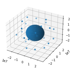
Ploting the 24 satellites of GPS
from mpl_toolkits.mplot3d import axes3d

# Create an array with the satellites position

fig = plt.figure()
ax = fig.add_subplot(111, projection='3d')

earth_diam = 2*6371E3

# Make data
u = np.linspace(0, 2 * np.pi, 100)
v = np.linspace(0, np.pi, 100)
x = earth_diam * np.outer(np.cos(u), np.sin(v))
y = earth_diam * np.outer(np.sin(u), np.sin(v))
z = earth_diam * np.outer(np.ones(np.size(u)), np.cos(v))

# Plot the surface
ax.plot_surface(x, y, z)

xs = []
ys = []
zs = []

satellite = GPS

for i in range(len(satellite.meanano)):

    eccen_ano = calc_eccen_ano(satellite.meanano[i], satellite.e)
    posVecAux = get_position_vector(satellite.a, satellite.e, eccen_ano)

    out = orbit_to_cis(satellite.argper, satellite.rightasc[i], satellite.i, posVecAux)

    xs.append(out[0])
    ys.append(out[1])
    zs.append(out[2])
    #ax.scatter(xs= out[0], ys= out[1], zs= out[2])
    #print("Satellite number {}: X{} Y{} Z{}".format(i, out[0], out[1], out[2]))

ax.scatter(xs, ys, zs)
plt.show()
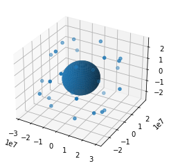
Plotting the 27 satellites of Galileo
import matplotlib.pyplot as plt
from mpl_toolkits.mplot3d import Axes3D

# Create an array with the satellites position

fig = plt.figure()
ax = fig.add_subplot(111, projection='3d')

earth_diam = 2*6371E3

# Make data
u = np.linspace(0, 2 * np.pi, 100)
v = np.linspace(0, np.pi, 100)
x = earth_diam * np.outer(np.cos(u), np.sin(v))
y = earth_diam * np.outer(np.sin(u), np.sin(v))
z = earth_diam * np.outer(np.ones(np.size(u)), np.cos(v))

# Plot the surface
ax.plot_surface(x, y, z)

xs = []
ys = []
zs = []

satellite = Galileo

for i in range(len(satellite.meanano)):

    eccen_ano = calc_eccen_ano(satellite.meanano[i], satellite.e)
    posVecAux = get_position_vector(satellite.a, satellite.e, eccen_ano)

    out = orbit_to_cis(satellite.argper, satellite.rightasc[i], satellite.i, posVecAux)

    xs.append(out[0])
    ys.append(out[1])
    zs.append(out[2])
    #ax.scatter(xs= out[0], ys= out[1], zs= out[2])
    #print("Satellite number {}: X{} Y{} Z{}".format(i, out[0], out[1], out[2]))

ax.scatter(xs, ys, zs)
plt.show()
Plot single GPS satellite for 12 hours
"""
Plot a single satellite for 12 hours
"""

hours = 12
samples = 200

"""
PLOT EARTH
"""
# Create an array with the satellites position

fig = plt.figure()
ax = fig.add_subplot(111, projection='3d')

# Plot earth
earth_diam = 2*6371E3

# Make data
u = np.linspace(0, 2 * np.pi, 100)
v = np.linspace(0, np.pi, 100)
x = earth_diam * np.outer(np.cos(u), np.sin(v))
y = earth_diam * np.outer(np.sin(u), np.sin(v))
z = earth_diam * np.outer(np.ones(np.size(u)), np.cos(v))

# Plot the surface
ax.plot_surface(x, y, z)

xs = []
ys = []
zs = []

satellite = GPS
sat_index = 0
for i in range(samples):
    inc_secs = ((hours*3600)/samples) * i

    delta = inc_secs * satellite.meanmotion
    mean_ano = satellite.meanano[sat_index] + delta
    eccen_ano = calc_eccen_ano(mean_ano, satellite.e)
    posVecAux = get_position_vector(satellite.a, satellite.e, eccen_ano)

    out = orbit_to_cis(satellite.argper, satellite.rightasc[sat_index], satellite.i, posVecAux)

    xs.append(out[0])
    ys.append(out[1])
    zs.append(out[2])

ax.scatter(xs, ys, zs)
plt.show()
Plot single Galileo satellite for 12 hours
"""
Plot a single satellite for 12 hours
"""

hours = 12
samples = 200

"""
PLOT EARTH
"""
# Create an array with the satellites position

fig = plt.figure()
ax = fig.add_subplot(111, projection='3d')

# Plot earth
earth_diam = 2*6371E3

# Make data
u = np.linspace(0, 2 * np.pi, 100)
v = np.linspace(0, np.pi, 100)
x = earth_diam * np.outer(np.cos(u), np.sin(v))
y = earth_diam * np.outer(np.sin(u), np.sin(v))
z = earth_diam * np.outer(np.ones(np.size(u)), np.cos(v))

# Plot the surface
ax.plot_surface(x, y, z)

xs = []
ys = []
zs = []

satellite = Galileo
sat_index = 0
for i in range(samples):
    inc_secs = ((hours*3600)/samples) * i

    delta = inc_secs * satellite.meanmotion
    mean_ano = satellite.meanano[sat_index] + delta
    eccen_ano = calc_eccen_ano(mean_ano, satellite.e)
    posVecAux = get_position_vector(satellite.a, satellite.e, eccen_ano)

    out = orbit_to_cis(satellite.argper, satellite.rightasc[sat_index], satellite.i, posVecAux)

    xs.append(out[0])
    ys.append(out[1])
    zs.append(out[2])

ax.scatter(xs, ys, zs)
plt.show()
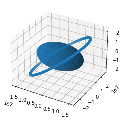
Plot all GPS satellites for 12 hours
"""
Plot a single satellite for 12 hours
"""


sat_index = 0
hours = 12
samples = 200

"""
PLOT EARTH
"""
# Create an array with the satellites position

fig = plt.figure()
ax = fig.add_subplot(111, projection='3d')

# Plot earth
earth_diam = 2*6371E3

# Make data
u = np.linspace(0, 2 * np.pi, 100)
v = np.linspace(0, np.pi, 100)
x = earth_diam * np.outer(np.cos(u), np.sin(v))
y = earth_diam * np.outer(np.sin(u), np.sin(v))
z = earth_diam * np.outer(np.ones(np.size(u)), np.cos(v))

# Plot the surface
ax.plot_surface(x, y, z)

xs = []
ys = []
zs = []

satellite = GPS

for sat_index in range(len(satellite.meanano)):
    xs = []
    ys = []
    zs = []

    for i in range(samples):
        inc_secs = ((hours*3600)/samples) * i

        delta = inc_secs * satellite.meanmotion
        mean_ano = satellite.meanano[sat_index] + delta
        eccen_ano = calc_eccen_ano(mean_ano, satellite.e)
        posVecAux = get_position_vector(satellite.a, satellite.e, eccen_ano)

        out = orbit_to_cis(satellite.argper, satellite.rightasc[sat_index], satellite.i, posVecAux)

        xs.append(out[0])
        ys.append(out[1])
        zs.append(out[2])


    ax.scatter(xs, ys, zs)
plt.show()
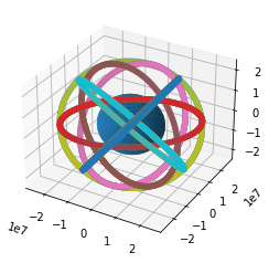
Plot all Galileo satellites for 12 hours
"""
Plot a single satellite for 12 hours
"""


sat_index = 0
hours = 12
samples = 200

"""
PLOT EARTH
"""
# Create an array with the satellites position

fig = plt.figure()
ax = fig.add_subplot(111, projection='3d')

# Plot earth
earth_diam = 2*6371E3

# Make data
u = np.linspace(0, 2 * np.pi, 100)
v = np.linspace(0, np.pi, 100)
x = earth_diam * np.outer(np.cos(u), np.sin(v))
y = earth_diam * np.outer(np.sin(u), np.sin(v))
z = earth_diam * np.outer(np.ones(np.size(u)), np.cos(v))

# Plot the surface
ax.plot_surface(x, y, z)

xs = []
ys = []
zs = []

satellite = Galileo

for sat_index in range(len(satellite.meanano)):
    xs = []
    ys = []
    zs = []

    for i in range(samples):
        inc_secs = ((hours*3600)/samples) * i

        delta = inc_secs * satellite.meanmotion
        mean_ano = satellite.meanano[sat_index] + delta
        eccen_ano = calc_eccen_ano(mean_ano, satellite.e)
        posVecAux = get_position_vector(satellite.a, satellite.e, eccen_ano)

        out = orbit_to_cis(satellite.argper, satellite.rightasc[sat_index], satellite.i, posVecAux)

        xs.append(out[0])
        ys.append(out[1])
        zs.append(out[2])


    ax.scatter(xs, ys, zs)
plt.show()
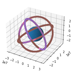
Evaluation of the previous plots
The previous plots looks very realistic, similar to the plots presented in the course slides
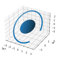
A plot showing the GPS positions in CIS over 12 hours using e=0.1
"""
Plot a single satellite for 12 hours
"""

hours = 12
samples = 200

"""
PLOT EARTH
"""
# Create an array with the satellites position

fig = plt.figure()
ax = fig.add_subplot(111, projection='3d')

# Plot earth
earth_diam = 2*6371E3

# Make data
u = np.linspace(0, 2 * np.pi, 100)
v = np.linspace(0, np.pi, 100)
x = earth_diam * np.outer(np.cos(u), np.sin(v))
y = earth_diam * np.outer(np.sin(u), np.sin(v))
z = earth_diam * np.outer(np.ones(np.size(u)), np.cos(v))

# Plot the surface
ax.plot_surface(x, y, z)

xs = []
ys = []
zs = []

satellite = GPS
sat_index = 0
e = 0.1
for i in range(samples):
    inc_secs = ((hours*3600)/samples) * i

    delta = inc_secs * satellite.meanmotion
    mean_ano = satellite.meanano[sat_index] + delta
    eccen_ano = calc_eccen_ano(mean_ano, e)
    posVecAux = get_position_vector(satellite.a, e, eccen_ano)

    out = orbit_to_cis(satellite.argper, satellite.rightasc[sat_index], satellite.i, posVecAux)

    xs.append(out[0])
    ys.append(out[1])
    zs.append(out[2])

ax.scatter(xs, ys, zs)
plt.show()
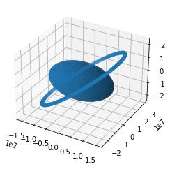
Evaluation and comparison with previous plots
In the previous plot we can appreciate the eccentricity of the orbit, I can consider the refresentation is correct. Comparing with the same satellite without this eccentricity we can see how the satellites is closer to the earth in the apogee.